UMN Projects
This records all projects done at the University of Minnesota
Stochastic Models for Intra-cellular Cargo Transport (2019)
Overall Goal:
- To model the cargo transport process as a combination of free diffusion and motor based transport
- Obtain time-evolution of the position and velocity of the cargo
- Get biologically relevant statistics using position and velocity evolution
Approach:
- Computational: Approximate numererical solutions to SDEs (e.g. Euler-Maruyama)
- Semi-Analytical: Use closed form solutions for each (sub)regime, combine them for faster computational solution
- Analytical: Attempt to find analytical solution to the joint SDEs with Poisson jumps and regime switching
The code can be found here.
Automating Flappy Bird using Deep Q-learning (2021)
Codes and reports can be seen here.
Here, we want to design an agent that can automate the flappy bird game based on state vectors instead of images, where the flappy Bird is a game that involves navigating a bird through a bunch of obstacles using reinforcement learning without knowing any information from the environment apriori.
Based on the rewards received, the agent learns to behave in a given environment under certain policy. Reinforcement Learning is mainly concerned with the maximization of cumulative reward in return to the agent-environment interaction. Deep Q-Learning is an advanced version of Q-Learning method of Reinforcement Learning where deep neural networks are used to solve Reinforcement Learning problems.
We attempted to automate the game flappy bird without giving the agent any environment related information except for rewards that it gets for different actions. The action value function was represented using a neural network and the network was trained using deep Q learning algorithm to store the Q values. Besides, we found out that our vector-based learning for flappy bird game is a little bit faster than the image-based one, which may give the intuition that we may decrease the information contained in the image further to get a better training speed since the image is constituted with vectors. So if we can find a proper method to do pre-processing on the image to keep the necessary information before training, we will have a better learning speed, and this is the work we want to study in details in the future.
gym-simpleflappy
A Gym environment for a Flappy bird clone with a simple observation space.
Observations returned are:
[bird height, bird speed, distance to next pipe, height of next pipe, distance to second pipe, height of second pipe]
Use gym.make("SimpleFlappy-v0") for rewards only when a pipe is passed.
Use gym.make("SimpleFlappyDistance-v0") for rewards based on steps survived - less sparse rewards should make the task a bit easier.
Run an Example
Run this sample agent (“flappy_random_agent.py”)to see the environment in action
This agent picks a random action (flap or not flap) every 15 frames. Score is printed after each episode.
Run the trained agent
Run the file “dqn_vector_flappyBird_final.py” to test the agent with pre-trained model.
Test video
A short test video is shown in “Test.MP4”, where the agent has scored more than 1500.
Score and Q(s,a)
These values are stored in “Q.txt” and “S.txt” for the last training.
Pretrained model
The pretrained model is saved in the folder “pretrained_model_vector”
Robust control for Self-erecting Inverted Pendulum (SESIP) (2020)
Codes and reports can be seen here.
The self-erecting single inverted pendulum (SESIP) is an unstable, multi-variable and fourth order system. We focus on the stabilizing and tracking control in this project.
In this project, the SESIP model is introduced first, then LQR control is applied with tracking the predetermined trajectory, stabilizing the inverted pendulum vertically and maintaining the input signal u(t) within 10V. Then we analyze LQR control with real uncertainty and multiplicative uncertainty. Last, we use H∞ and μ-synthesis control to further analyze the robustness and performance characteristics of the system.
First, we implemented the double PID control, while the double PID control is not good to use. Therefore we change to the LQR control, we first use simple LQR, but the input signal is too large, which exceeds our limitation. Due to this reason, we add extra weighting term on our input signal.
Then, we test the robust stability of controller with real uncertainty and dynamic uncertainty. And we can conclude that LQR control has a very good robustness on real uncertainties, but it has a weak robustness on multiplicative uncertainty. Besides, we found that the LQR control without limitation on u(t) will give stronger robustness on multiplicative uncertainty compared with LQR with limitation on u(t). It’s probably because limitation on u(t) gives up some robust stability and we need to clarify it in the future.
Last, we move to H∞ and μ-synthesis control to get a more robust controller based on the multiplicative uncertainty and try to do model reduction on kμ to make it more applicable in the real world. However, we don’t go deep in the model reduction method here, and it’s still unclear why the reduced controller with order 11 will give lower bound 0, which needs future work as well.
- Please see more details in “Robust control for Self-erecting Inverted Pendulum.pdf”
- Codes and how to use them can be seen in “Pendulum_lqr.pdf”, “pendulum_hinf.pdf” and “pendulum_uncertainty.pdf”
A Research on Performance Discrepancy for Varying Fine-tuning Layers and Pooling Strategies of BERT (2021)
Codes and reports can be seen here.
The goal of this project is to investigate how different fine-tuning layers and pooling strategies will influence the performance of transformer based model. Specifically, we used BERT as our experimental model.
We attempted to use two dimensional Convolutional Neural Networks (CNN2D), one dimensional Convolutional Neural Networks (CNN1D) and Bidirectional Long-Short Term Memory (BiLSTM) to fine tune the hidden states from different layers, we need to construct the hidden states that can be fed into the fine tune layers in different ways.
For performance measure, two metrics accuracy and F1 score are used.
From this project, we found that it’s possible to improve performance when different kinds of finetune layers are added for information post-processing from hidden states of BERT. Specifically, even though original method(FC pooler layer with FC finetune layer) proposed by the paper give relatively promising performance, the best combination(CNN2D pooler layer with CNN2D finetune layer) we attempted can achieve marginal improvement on top of the original method on both Accuracy and F1 scores.
Please see PDF for more information!
Machine Learning Algorithms From Scratch (2021)
Codes and reports can be seen here.
These are some machine learning algorithms, which are coded from scratch that can be useful to help understand the mechanism and mathematics behind them.
LDA1dThres.py: Fisher’s linear discriminant analysis (LDA) with threshold
The input argument is the number of folds in cross-validation, which should be integer larger than 1. And the default value for the input argument is 10.
LDA2dGaussGM.py: LDA with bi-variate Gaussian generative modeling
We use two methods: shared covariance matrix and covariance matrix. In this code, it uses the shared covariance matrix method. If you want to see what’s going on with the other method, in the code you can comment the line with “covariance_sum” out , and comment the following line in.
Like LDA1dThres, the input is the same and default value is 10.
logisticRegression.py: Logistic regression (LR)
The function here takes three input arguments, one is num_splits(integer) with default value 10, and the other is train_percent(list of integer), with default value [10,25,50,75,100]. Besides, in order to choose which dataset we are going to use, I add one another input argument data_choose with default value to be 1, If data_choose = 1, then we choose Boston50, if data_choose = 2, then we choose Boston75, if data_choose =3, then we choose Digits. And values except mentioned the mentioned above three are invalid.
naiveBayesGaussian.py: Naive-Bayes with marginal Gaussian distributions (GNB)
The input argument have the same format and meaning as we discussed in logisticRegression.py.
SVM_dual.py: A linear SVM in dual form
The function SVM_dual(dataset = “/Desktop/CSCI5525/HW/HW2/hw2_data_2020.csv”), the input argument is the route of where the data is located on my computer, if you want to test the function on your side, remember to change the route of the dataset and then run the function.
kernel_SVM.py: Kernel SVM
kernel_SVM(dataset = “/Desktop/CSCI5525/HW/HW2/hw2_data_2020.csv”), need to change the input argument.
multi_SVM.py: A multi-class SVM using the one vs all strategy.
The function takes the form: multi_SVM(dataset = “/Desktop/CSCI5525/HW/HW2/mfeat”), which has similar explanation with before. Besides, only need the name “mfeat” here then I will combine all 6 dataset in the code. Note that if you run multi_SVM, then the function will process the part with linear kernel and print out the desired stuffs, then it will continue to run the second part with RBF kernel and then print out stuffs.
neural_net.py: A multi-layer fully connected neural network:
Just call the function neural_net() to get the result. The cumulative training loss and accuracy is been placed in the list for all epochs.
cnn.py: A convolutional neural network
Just call the function cnn() to get results.
adaboost.py: Implement the Adaboost algorithm with 100 weak learners and apply it to the cancer dataset
The function adaboost(dataset = “/Users/huacailong/Desktop/CSCI5525/HW/HW4/breast-cancer-wisconsin.data”), the input argument is the route of where the data is located on my computer, if you want to test the function on your side, remember to change the route of the dataset and then run the function.
rf.py: Implement the Random Forest algorithm with 100 decision stumps.
The function here is similar with problem 1 and takes the form: rf(dataset = “/Users/huacailong/Desktop/CSCI5525/HW/HW4/breast-cancer-wisconsin.data”), need to change the input argument as the same way in adaboost.py
kmeans.py: Implement the k-means algorithm and apply it to the image “umn csci.png”
The function takes the form: kmeans(image = “/Users/huacailong/Desktop/CSCI5525/HW/HW4/umn_csci.png”), need to change the input argument as the same way in adaboost.py.
Control Systems, Artificial Intelligence and Reinforcement Learning related topics (2021)
Robust Control
Robust control methods/algorithms applied on different systems, please the corresponding PDF for more details in the code here.
Nonlinear Control
Solved some nonlinear control problem here, please see codes and corresponding PDF for more details here.
Optimal Filtering
Have coded well-known algorithms in optimal filtering, like Linear Estimator, Least Square Estimator, Monte Carlo Method, Kalman Filter, Extended Kalman Filter, etc. Please see details in the code and corresponding PDF files here.
Artificial Intelligence and Reinforcement Learning
All codes are in Jupyter Notebook here. You can see more details and instructions once you opened them.
Computer Vision Related Problem (2022)
Wrote codes from scratch to deal with the computer vision related problems, the code can be found here.
- HOG: Please see HOG.py and HOG.pdf for details. The used figures are in the folder HOG Figures
- Implement a variant of HOG (Histogram of Oriented Gradi- ents) in Python proposed by Dalal and Trigg [1] (2015 Longuet-Higgins Prize Winner).
- Using the HOG descriptor, design a face detection algorithm.
- Registration: Please see Registration.py and Registration.pdf for details. The used figures are in the folder Registration Figures
- SIFT visualization, extraction and feature matching
- Compute an affine transform using SIFT matches filtered by RANSAC.
- Affine transform to warp the target image to the template using the inverse mapping.
- Inverse Compositional Image Alignment to update the affine transform
- Track over frames using the inverse compositional image alignment.
- Scene Recognition: Please see scene_recognition.py and scene_recognition.pdf for details. The used datasets are in the folder scene_classification_data
- Compute a set of image representations (tiny image and bag-of-word visual vocabulary)
- Predict the category of each testing image using the classifiers (k-nearest neighbor and SVM) built on the training data.
- Build a set of visual recognition systems that classify the scene categories.
- Convolutional Neural Network: Please see cnn.py, main_functions.py and Convolutional Neural Network.pdf for details. The used datasets are in the folder Convolutional Neural Network
- Implement neural network to recognize hand-written digits in the MNIST data.
- Implement a single-layer linear perceptron with stochastic gradient descent method.
- Implement a single-layer perceptron with soft-max cross-entropy using stochas- tic gradient descent method.
- Implement a multi-layer perceptron with a single hidden layer using a stochastic gradient descent method.
- Implement a convolutional neural network (CNN) using a stochastic gradient descent method.
- Stereo_Reconstruction: Please see Stereo_Reconstruction.py and Stereo_Reconstruction.pdf for details. The used figures are in the folder Stereo_Reconstruction_Figures
- Match points between two images using SIFT features.
- Compute a fundamental matrix to draw epipolar lines.
- Given camera pose and correspondences, triangulate to reconstruct 3D points.
- Find the best camera pose by verifying through 3D point triangulation.
- Implement dense stereo matching be- tween two views based on dense SIFT.
Langevin-based Sampling Algorithms with Energy-Based Models (2022)
Codes and thesis can be seen here.
Energy based Models(EBMs)
Energy-based model (EBM) is an approach designed to estimate the probability density. Energy-based models are prevalent in recent studies and are useful in image generation problems. However, the intractable partition function makes the training procedure of EBMs challenging and the current solution is to sampling methods to approximate the expectation in the maximum likelihood loss function.
Langevin-Based Sampling Methods
Different sampling methods are used to draw samples from the target distribution.
- (1) Stochastic Gradient Langevin Approach (SGLA) is a sampling technique that fuse the characteristics from stochastic gradient descent (SGD) and Langevin dynamics, which is a mathematical extension of molecular dynamics models.
- (2) Projected stochastic gradient Langenvin algorithm (PSGLA) takes constraints into consideration.
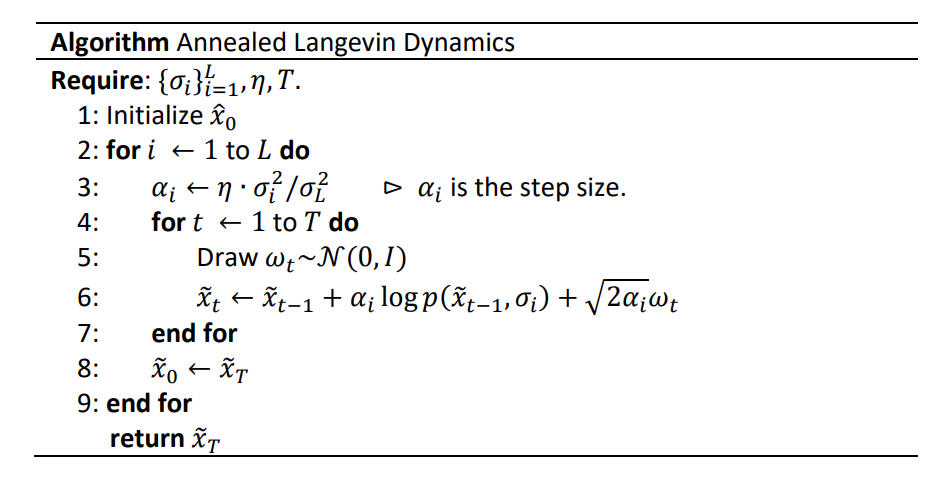
- (3) Annealed Langevin Algorithm (ALA) do SGLA in annealed way, where the initialization for current simulation is the final point from previous simulation.
Results: 2-D localization problem
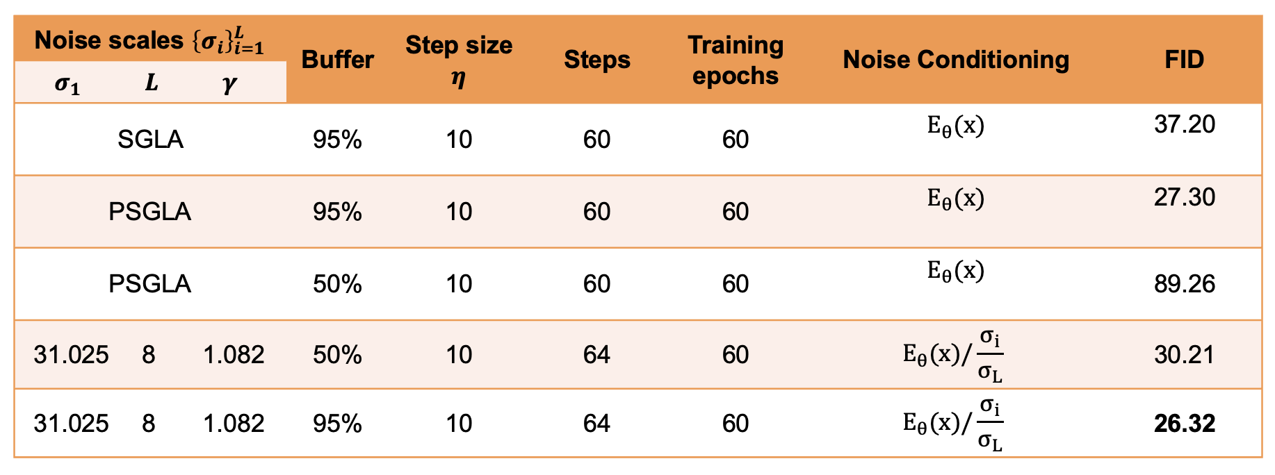
Then different Langevin-based sampling methods are studied and implemented on a simple 2-D localization problem and results show that the PSGLA is better than the SGLA with engaging constraints.
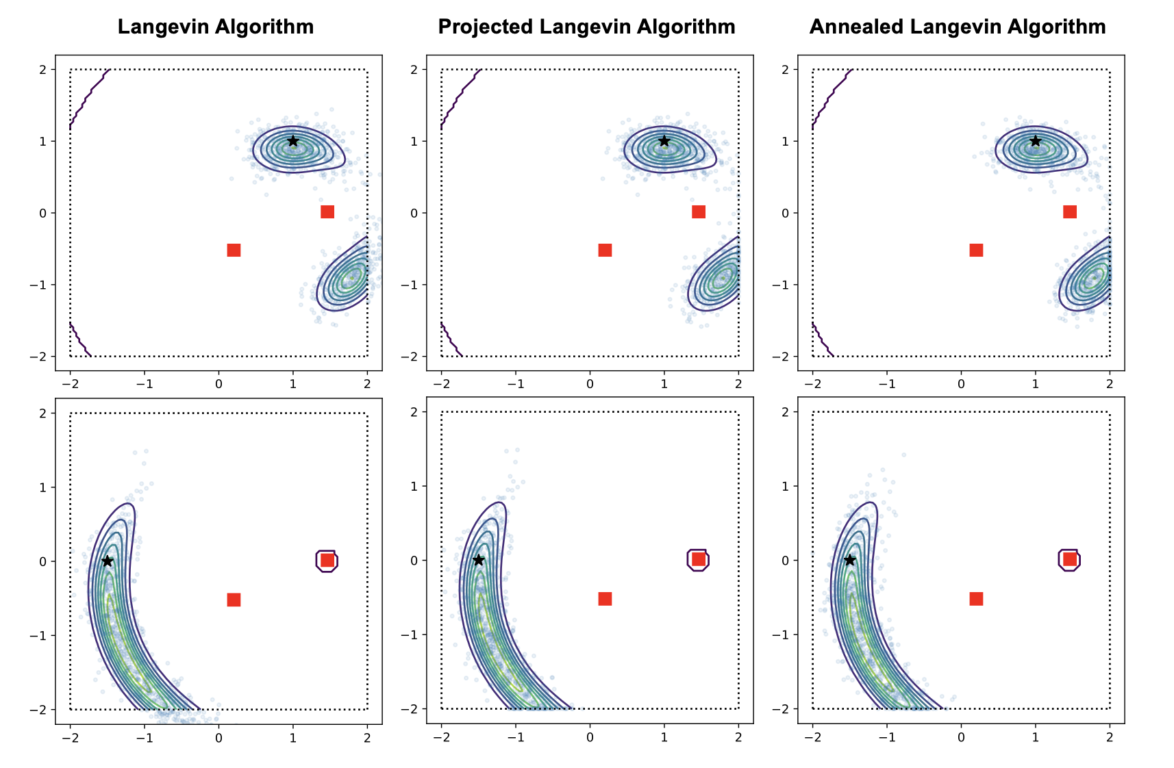
Annealed Langevin algorithm performs better than PSGLA when the distribution is unbalanced due to the intrinsic initialization advantage in Annealed Langevin algorithm.
Results: EBMs with MNIST dataset
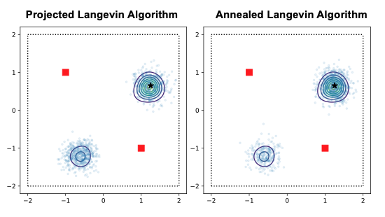
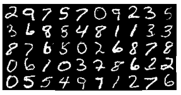
Moreover, we trained EBM with three different sampling methods on MNIST dataset. We can conclude 1) constraints are crucial in the sampling methods since they will limit the generated image in the correct domain; 2) a good initialization is crucial to the sampling methods, where Annealed Langevin algorithm has its own method to do initialization while PSGLA needs the additional initialization buffer. Besides the good initialization method in Annealed Langevin algorithm, it also performs better in the unbalanced distribution and this advantage is not fully exploited using the MNIST dataset. The qualatitive and quantative results can be seen in the following.
HUMBI: Pose-Guided Human Rendering Challenge (2022)
Codes and thesis can be seen here. Pose-guided person image generation, which is to synthesize a realistic image of the person with the target pose based on a source image showing the person with a given pose, has attracted much attention recently.
For more details, please see “HUMBI_Pose-Guided Human Rendering Challenge.pdf”.
Baseline: XingGAN See here
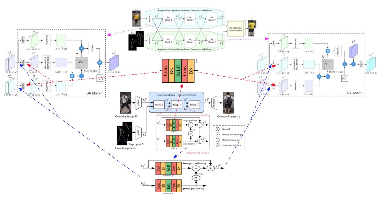
And the generator aims to synthesize realistic person image, which is transferred from the person in source image with source pose to target pose. The Xing generator has three major components:
- (1) Shape-guided Appearance-based generation (SA) branch to model the person shape representation based on an input of appearance representation;
- (2) Appearance-guided Shape-based generation (AS) branch to model the person appearance representation based on an input of shape representation;
- (3) Co-Attention Fusion (CAF) module for fusing the two branches to generate the syn- thesized image using the both appearance and shape codes.
The SA branch and AS branch contains identical cascaded SA blocks and AS blocks correspondingly and the appearance code and shape code are updated in a cross-conditioning strategy under the guidance of each other.
Dataset: HUMBI dataset
HUMBI dataset is available at http://humbi-data.net/ and there is a benchmark challenge open for participation. This project aims to compete for this chal- lenge using proposed method based on XingGAN.
Method: XingGAN and Pose-Transfer
Therefore, our proposed solution is to come up with a hybrid model by combining the pose transfer framework with the baseline aiming to get a performance improvement. To figure out what leads to higher pose consistence, we first added two neural networks in each SA and AS block, which can be seen as the red dashed lines in following figure and then added image code update part in PATB previous to SA and AS block, which can be seen as the blue dashed lines in following figure.
Results: quantitative and qualitative results.
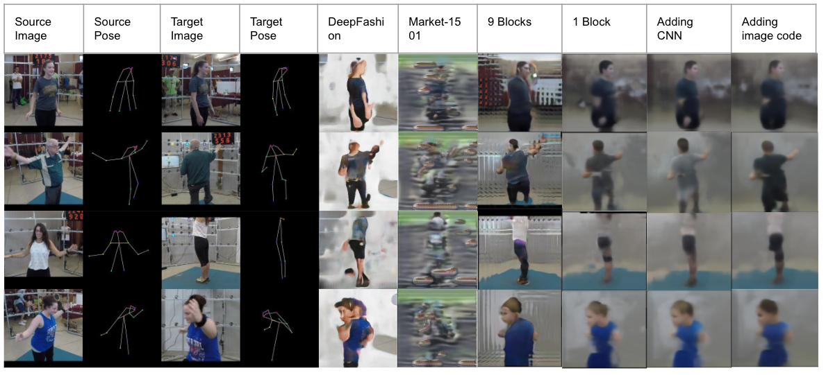
In total, XingGAN with CNN has the best performance over all and XingGAN with image code update and XingGAN with 1 block have similar performance, which are slightly worse than XingGAN with CNN.
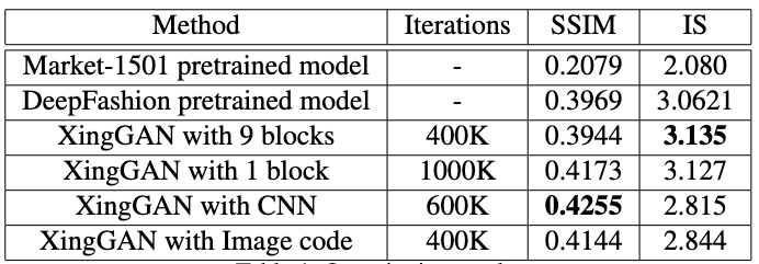
In total, XingGAN with CNN yields the best similarity between the targe images and synthesized images and XingGAN with 9 blocks has the best inception score.
Discussion:
- From both quantitative and qualitative results, we were surprised that the both IS and SSIM are only around 0.3 and the synthesized images are not clear.
- We found that XingGAN can achieve SSIM more than 0.7 for Deep- Fashion dataset, where the background is white only, but XingGAN achieves SSIM score around 0.3 for the market-1501 dataset, where the background is composed with details, for examples, trees, bikes and other persons.
- The reason why XingGAN achieves a lower score for Market-1501 is the score is impaired by the unclear background, where the XingGAN method is not good at.
- And in our HUMBI dataset, we have both person and the background, even though we have a good pose transfer for the person, but we are not very good at transferring the background so that our SSIM is also low, which is around 0.4. In conclusion, XingGAN is good at pose transfer but not good at backgrounds.
How to use:
- Download the dataset from http://humbi-data.net/ and unzip it into the folder SelectionGAN/person_transfer/datasets/humbi_data
- Generate pose map files (.npy files) using python files in SelectionGAN/person_transfer/datasets
- Use “XingGAN_train_modified_1”, “XingGAN_train_modified_2”,”XingGAN_train_original_1” and “XingGAN_train_original_2” to train the XingGAN under different settings. Or you can download the pretrained model at https://drive.google.com/drive/folders/1Ebu_06nc3B_TKQYYLepK-QbM1Cm0W_OU?usp=sharing.
- Then use those test python files to test your trained XingGAN on the HUMBI dataset, the result is available in the folder results/
- Then use tool/getMetrics_humbi_9blocks.py to get the scores.
Causality for Protein Modelling (2022)
- Uncovered causal relations from protein pulling data
- Quantified the change of effects among protein properties
- Examined both above questions assuming the existence of unobserved data.